ISBI 2012 Simple 2D Multicut Pipeline

Here we segment neuro data as in [BPR+17]. In fact, this is a simplified version of [BPR+17]. We start from an distance transform watershed over-segmentation. We compute a RAG and features for all edges. Next, we learn the edge probabilities with a random forest classifier. The predicted edge probabilities are fed into multicut objective. This is optimized with an ILP solver (if available). This results into a ok-ish learned segmentation for the ISBI 2012 dataset.

This example will download a about 400 MB large zip file with the dataset and precomputed results from [BPR+17]

# multi purpose
import numpy
import scipy

# plotting
import pylab

# to download data and unzip it
import os
import urllib.request
import zipfile

# to read the tiff files
import skimage.io
import skimage.filters
import skimage.morphology

# classifier
from sklearn.ensemble import RandomForestClassifier

# needed parts of nifty
import nifty
import nifty.segmentation
import nifty.filters
import nifty.graph.rag
import nifty.ground_truth
import nifty.graph.opt.multicut

Download ISBI 2012:

Download the ISBI 2012 dataset and precomputed results form [BPR+17] and extract it in-place.

fname = "data.zip"
url = "http://files.ilastik.org/multicut/NaturePaperDataUpl.zip"
if not os.path.isfile(fname):
    urllib.request.urlretrieve(url, fname)
    zip = zipfile.ZipFile(fname)
    zip.extractall()

Setup Datasets:

load ISBI 2012 raw and probabilities for train and test set and the ground-truth for the train set

rawDsets = {
    'train' : skimage.io.imread('NaturePaperDataUpl/ISBI2012/raw_train.tif'),
    'test' : skimage.io.imread('NaturePaperDataUpl/ISBI2012/raw_test.tif'),
}
# read pmaps and convert to 01 pmaps
pmapDsets = {
    'train' : skimage.io.imread('NaturePaperDataUpl/ISBI2012/probabilities_train.tif'),
    'test' : skimage.io.imread('NaturePaperDataUpl/ISBI2012/probabilities_test.tif'),
}
pmapDsets = {
    'train' : pmapDsets['train'].astype('float32')/255.0,
    'test' : pmapDsets['test'].astype('float32')/255.0
}
gtDsets = {
    'train' : skimage.io.imread('NaturePaperDataUpl/ISBI2012/groundtruth.tif'),
    'test'  : None
}

computedData = {
    'train' : [{} for z in range(rawDsets['train'].shape[0])],
    'test'  : [{} for z in range(rawDsets['test'].shape[0])]
}

Helper Functions:

Function to compute features for a RAG (used later)

def computeFeatures(raw, pmap, rag):

    uv = rag.uvIds()
    nrag = nifty.graph.rag

    # list of all edge features we fill
    feats = []

    # helper function to convert
    # node features to edge features
    def nodeToEdgeFeat(nodeFeatures):
        uF = nodeFeatures[uv[:,0], :]
        vF = nodeFeatures[uv[:,1], :]
        feats = [ numpy.abs(uF-vF), uF + vF, uF *  vF,
                 numpy.minimum(uF,vF), numpy.maximum(uF,vF)]
        return numpy.concatenate(feats, axis=1)


    # accumulate features from raw data
    fRawEdge, fRawNode = nrag.accumulateStandartFeatures(rag=rag, data=raw,
        minVal=0.0, maxVal=255.0, numberOfThreads=1)
    feats.append(fRawEdge)
    feats.append(nodeToEdgeFeat(fRawNode))

    # accumulate data from pmap
    fPmapEdge, fPmapNode = nrag.accumulateStandartFeatures(rag=rag, data=pmap,
        minVal=0.0, maxVal=1.0, numberOfThreads=1)
    feats.append(fPmapEdge)
    feats.append(nodeToEdgeFeat(fPmapNode))

    # accumulate node and edge features from
    # superpixels geometry
    fGeoEdge = nrag.accumulateGeometricEdgeFeatures(rag=rag, numberOfThreads=1)
    feats.append(fGeoEdge)

    fGeoNode = nrag.accumulateGeometricNodeFeatures(rag=rag, numberOfThreads=1)
    feats.append(nodeToEdgeFeat(fGeoNode))

    return numpy.concatenate(feats, axis=1)

Over-segmentation, RAG & Extract Features:

Compute:

• Over-segmentation with distance transform watersheds.
• Construct a region adjacency graph (RAG)
• Extract features for all edges in the graph
• Map the ground truth to the edges in the graph. (only for the training set)

for ds in ['train', 'test']:

    rawDset = rawDsets[ds]
    pmapDset = pmapDsets[ds]
    gtDset = gtDsets[ds]
    dataDset = computedData[ds]

    # for each slice
    for z in range(rawDset.shape[0]):


        data = dataDset[z]

        # get raw and pmap slice
        raw  = rawDset[z, ... ]
        pmap = pmapDset[z, ... ]



        # oversementation
        overseg = nifty.segmentation.distanceTransformWatersheds(pmap, threshold=0.3)
        overseg -= 1
        data['overseg'] = overseg

        # region adjacency graph
        rag = nifty.graph.rag.gridRag(overseg)
        data['rag'] = rag

        # compute features
        features = computeFeatures(raw=raw, pmap=pmap, rag=rag)

        data['features'] = features

        # map the gt to edge
        if ds == 'train':

            # the gt is on membrane level
            # 0 at membranes pixels
            # 1 at non-membrane pixels
            gtImage = gtDset[z, ...]

            # local maxima seeds
            seeds = nifty.segmentation.localMaximaSeeds(gtImage)

            # growing map
            growMap = nifty.filters.gaussianSmoothing(1.0-gtImage, 1.0)
            growMap += 0.1*nifty.filters.gaussianSmoothing(1.0-gtImage, 6.0)
            gt = nifty.segmentation.seededWatersheds(growMap, seeds=seeds)


            # map the gt to the edges
            overlap = nifty.ground_truth.overlap(segmentation=overseg,
                                       groundTruth=gt)

            # edge gt
            edgeGt = overlap.differentOverlaps(rag.uvIds())
            data['edgeGt'] = edgeGt


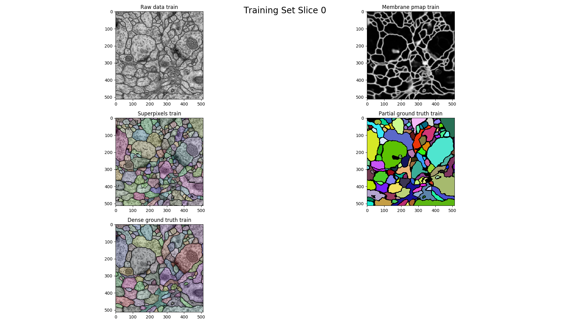
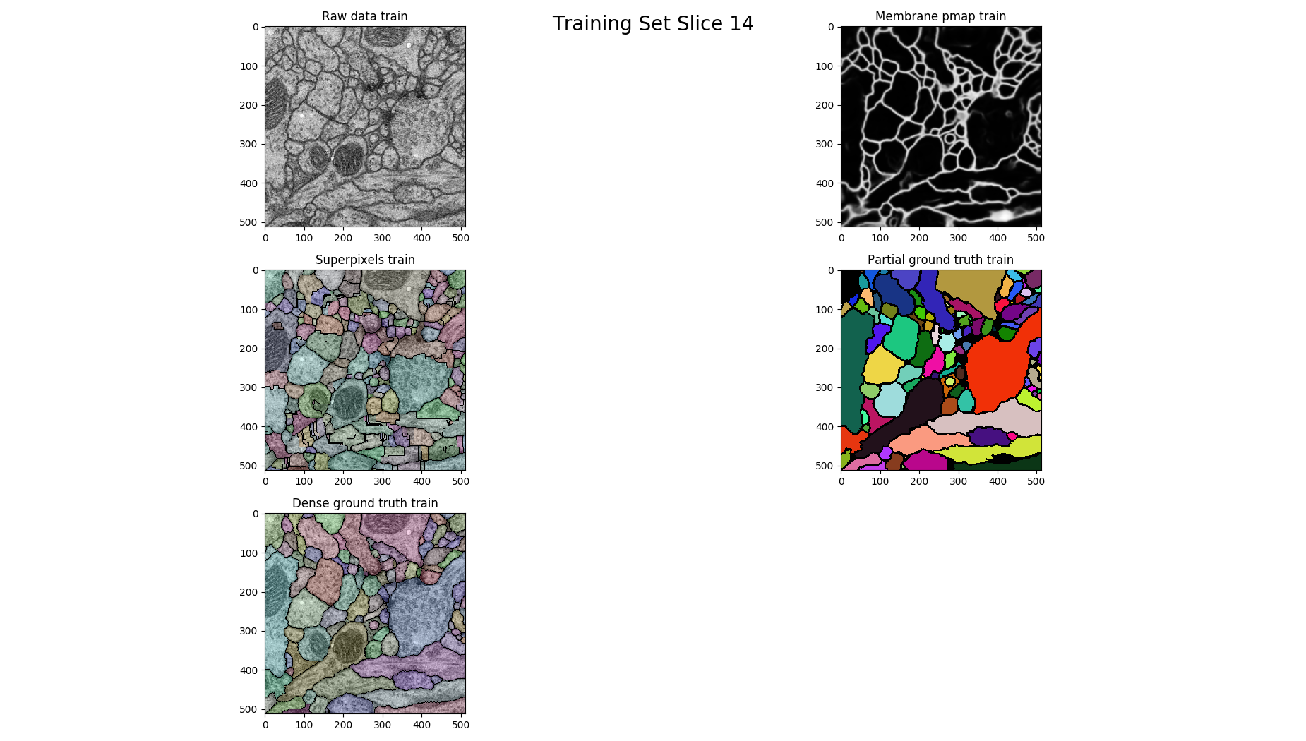
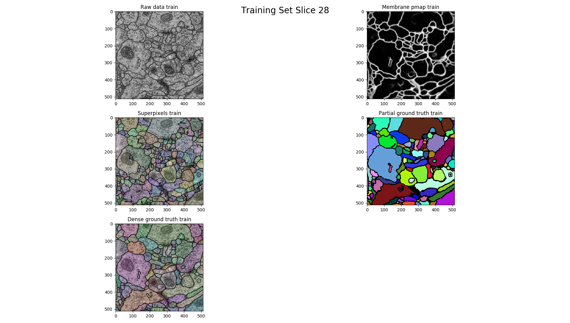
            # plot each 14th
            if z  % 14 == 0 :
                figure = pylab.figure()
                figure.suptitle('Training Set Slice %d'%z, fontsize=20)

                #fig = matplotlib.pyplot.gcf()
                figure.set_size_inches(18.5, 10.5)

                figure.add_subplot(3, 2, 1)
                pylab.imshow(raw, cmap='gray')
                pylab.title("Raw data %s"%(ds))

                figure.add_subplot(3, 2, 2)
                pylab.imshow(pmap, cmap='gray')
                pylab.title("Membrane pmap %s"%(ds))


                figure.add_subplot(3, 2, 3)
                pylab.imshow(nifty.segmentation.segmentOverlay(raw, overseg, 0.2, thin=False))
                pylab.title("Superpixels %s"%(ds))

                figure.add_subplot(3, 2, 4)
                pylab.imshow(seeds, cmap=nifty.segmentation.randomColormap(zeroToZero=True))
                pylab.title("Partial ground truth %s" %(ds))

                figure.add_subplot(3, 2, 5)
                pylab.imshow(nifty.segmentation.segmentOverlay(raw, gt, 0.2, thin=False))
                pylab.title("Dense ground truth %s" %(ds))
                pylab.tight_layout()
                pylab.show()

        else:
            data['edgeGt'] = None

• 
• 
• 

Build the training set:

We only use high confidence boundaries.

dataDset = computedData[ds]
trainingSet = {'features':[],'labels':[]}

for ds in ['train']:

    rawDset = rawDsets[ds]
    pmapDset = pmapDsets[ds]
    gtDset = gtDsets[ds]
    dataDset = computedData[ds]

    # for each slice
    for z in range(rawDset.shape[0]):

        data = dataDset[z]

        rag = data['rag']
        edgeGt = data['edgeGt']
        features = data['features']

        # we use only edges which have
        # a high certainty
        where1 = numpy.where(edgeGt > 0.85)[0]
        where0 = numpy.where(edgeGt < 0.15)[0]

        trainingSet['features'].append(features[where0,:])
        trainingSet['features'].append(features[where1,:])
        trainingSet['labels'].append(numpy.zeros(len(where0)))
        trainingSet['labels'].append(numpy.ones(len(where1)))

features = numpy.concatenate(trainingSet['features'], axis=0)
labels = numpy.concatenate(trainingSet['labels'], axis=0)

Train the random forest (RF):

rf = RandomForestClassifier(n_estimators=200, oob_score=True)
rf.fit(features, labels)
print("OOB SCORE",rf.oob_score_)

Out:

OOB SCORE 0.981860916662

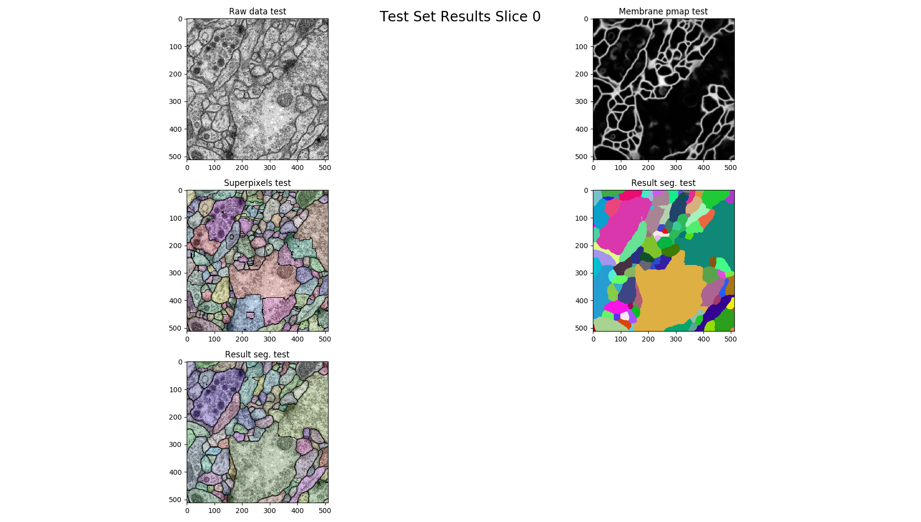
Predict Edge Probabilities & Optimize Multicut Objective:

Predict the edge probabilities with the learned random forest classifier. Set up a multicut objective and find the argmin with an ILP solver (if available).

for ds in ['test']:

    rawDset = rawDsets[ds]
    pmapDset = pmapDsets[ds]
    gtDset = gtDsets[ds]
    dataDset = computedData[ds]

    # for each slice
    for z in range(rawDset.shape[0]):


        data = dataDset[z]

        raw = rawDset[z,...]
        pmap = pmapDset[z,...]
        overseg = data['overseg']
        rag = data['rag']
        edgeGt = data['edgeGt']
        features = data['features']

        predictions = rf.predict_proba(features)[:,1]


        # setup multicut objective
        MulticutObjective = rag.MulticutObjective

        eps =  0.00001
        p1 = numpy.clip(predictions, eps, 1.0 - eps)
        weights = numpy.log((1.0-p1)/p1)




        objective = MulticutObjective(rag, weights)

        # do multicut obtimization
        if nifty.Configuration.WITH_CPLEX:
            solver = MulticutObjective.multicutIlpCplexFactory().create(objective)
        elif nifty.Configuration.WITH_GUROBI:
            solver = MulticutObjective.multicutIlpGurobiFactory().create(objective)
        else:
            solver = MulticutObjective.ccFusionMoveBasedFactory().create(objective)


        arg = solver.optimize(visitor=MulticutObjective.verboseVisitor())
        result = nifty.graph.rag.projectScalarNodeDataToPixels(rag, arg)


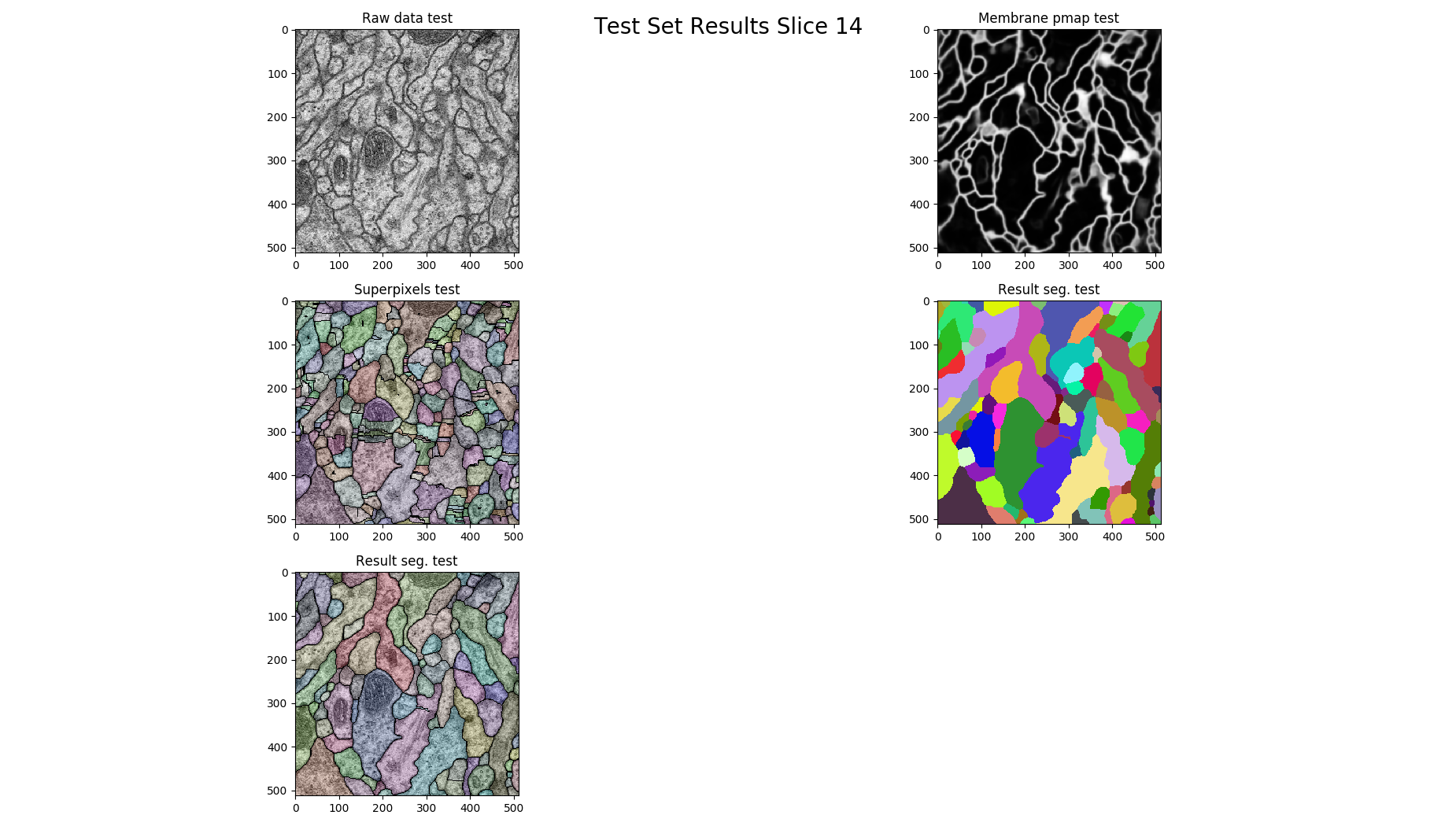
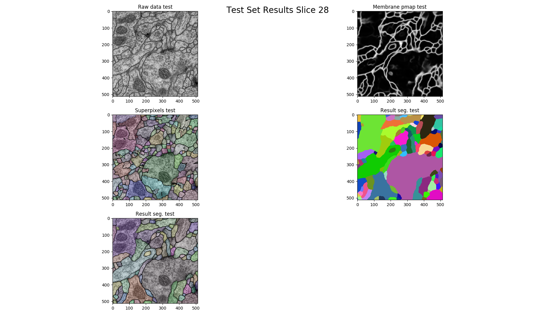
        # plot for each 14th slice
        if z % 14 == 0:
            figure = pylab.figure()

            figure.suptitle('Test Set Results Slice %d'%z, fontsize=20)

            #fig = matplotlib.pyplot.gcf()
            figure.set_size_inches(18.5, 10.5)

            figure.add_subplot(3, 2, 1)
            pylab.imshow(raw, cmap='gray')
            pylab.title("Raw data %s"%(ds))

            figure.add_subplot(3, 2, 2)
            pylab.imshow(pmap, cmap='gray')
            pylab.title("Membrane pmap %s"%(ds))


            figure.add_subplot(3, 2, 3)
            pylab.imshow(nifty.segmentation.segmentOverlay(raw, overseg, 0.2, thin=False))
            pylab.title("Superpixels %s"%(ds))

            figure.add_subplot(3, 2, 4)
            pylab.imshow(result, cmap=nifty.segmentation.randomColormap())
            pylab.title("Result seg. %s" %(ds))

            figure.add_subplot(3, 2, 5)
            pylab.imshow(nifty.segmentation.segmentOverlay(raw, result, 0.2, thin=False))
            pylab.title("Result seg. %s" %(ds))
            pylab.tight_layout()
            pylab.show()

• 
• 
• 

Total running time of the script: ( 2 minutes 15.624 seconds)